Discretization Error amplification instead of stagnation to machine precision

Question

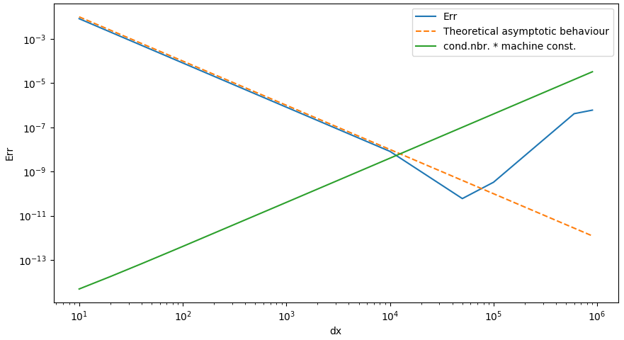
I wrote a code on Python 2.7.5 to solve numerically the following differential equation.

• $\frac{\partial^2f}{\partial x^2}=-S$

• $S=\pi^{2}\sin(\pi x)$

S is chosen that way in order to have $f= \sin(\pi x)$ as the exact solution, that can be compared with the constructed solution.

The differential operator is discretized using a second-order central finite difference method.

When running the code, the order of magnitude of the evolution of the discretization error Err is correct (2nd order) for the first batch of points of N (10,20,40,80,100,800,2000,5000) (goes down to 10e-11).

But I found that for very small dx meaning, very big Nx (10000,50000,100000,600000,900000), Err doesn't stagnate at the machine precision error (as expected) but goes up for several magnitude orders, and even worse, the discretization error Err deteriorates (up to 10e-7).

Is it a problem in the precision/round managment of Python for very small numbers, or is it normal to have even worse Error for that amount of points ?

I tried to write the problem in different ways (Matrix, Loops, Matrix inversion technices) but the same phenomenon happened.

import numpy as np
import matplotlib.pyplot as plt
import scipy.sparse as sp
from scipy.sparse.linalg.dsolve import spsolve

Err=[]
N=np.array([10,20,40,80,100,800,2000,5000,10000,50000,100000,600000,900000])

#Loop on the number of points used for the discretization of the 1D domain   
for Nx in N:

    dx=(1.0)/Nx# fixed distance between two consecutive points in the domain
    x = np.linspace(dx,1.0-dx,Nx-1)# points of the 1D domain


    #contruction of the diff operator discretization Matrix
    data = [np.ones(Nx-1), -2*np.ones(Nx-1), np.ones(Nx-1)]# Diagonal terms
    offsets = np.array([-1, 0, 1])# Their positions
    LAP = sp.dia_matrix((data, offsets), shape=(Nx-1, Nx-1))#Sparse matrix
    S = np.pi**2*np.sin(np.pi*x)*dx**2# Second member 
    f = spsolve(LAP,-S)#Resolution of the matrix system 

    f_ana=np.sin(np.pi*x)#The exact solution

    Err.append((np.absolute((f_ana-f))).max())

plt.figure()
plt.plot(N,Err,N,N**float(-2),'--')
plt.legend(['Err','Theoretical asymptotic behaviour'])
plt.xlabel('dx')
plt.ylabel('Err')
plt.xscale('log')
plt.yscale('log')
plt.show()

Answer 1

Putting a more systematic point of view to the particular problems in the answer of H. Rittich, the matrices LAP are nearly singular for large N.

The eigensystem $$ v_{k-1}-2v_k+v_{k+1}=\lambda v_k,~~v_0=v_{N+1}=0 $$ has basis solutions $v_k=q^k-q^{-k}$ where $q^{2N+2}=1$ for $v_{N+1}=0$. Then the eigenvalue computes as $\lambda=q+q^{-1}-2$, which means $$ q_m=\exp(i\frac{m\pi}{N+1}),\\ v_{m,k}=2\cos(\frac{km\pi}{N+1}),\\ \lambda_m=2(\cos(m\frac{\pi}{N+1})-1)=-4\sin^2(\frac{m\pi}{2(N+1)}) $$ for $m=1,...,N$. Thus the ratio of largest to smallest eigenvalue, in other words the condition number of LAP, is $$ \kappa({\sf LAP})=\frac{\sin^2(\frac{N\pi}{2(N+1)})}{\sin^2(\frac{\pi}{2(N+1)})}\approx \frac{4(N+1)^2}{\pi^2}. $$ Floating point noise gets magnified by that number in the relative error formula, see the general perturbation theory of linear systems. This already includes effects of catastrophic cancellation.

As one can see, the truncation error stops to be close to the observed error at the point that the (theoretically possible magnitude of the) magnified floating point noise starts to dominate the truncation error.

Answer 2

Yes. This behavior is to be expected and normal. When you are computing with a small value for $\mathrm dx$ then, to compute the difference quotient, you are subtracting two numbers that are nearly the same. In this situation, you observe a so called catastrophic cancellation, meaning nearly all significant digits are lost (see here).

Answer 3

@H.Rittich states one reason in their answer. Another reason is that when you go to more and more points, you have to do more and more computations, each of which adds its own amount of round-off error. Consequently, the smaller your $\delta x$ gets, the more computations and the more accumulated round-off -- it doesn't just stay constant, but actually grows.