Oscillation in non-linear porous flow solved by finite difference

Question

I am trying to solve numerically the flow of a gas through a porous, spherically symmetric body. The non-dimensional equations read: $$ \frac{\partial\rho}{\partial t}+\tau\frac{1}{r^2}\frac{\partial}{\partial r}\left(r^2\rho v\right)=g_P\\ v=-\frac{\partial \rho}{\partial r}\\ $$ where $\rho$ is the gas density, $t$ time, $r$ radius (between $0$ and outer radius $R_p$), $v$ gas (radial) velocity, $g_P$ gas production rate, and $\tau$ a non-dimensional parameter accounting for permeability among other things (actually all quantities are non-dimensional). Essentially, the first equation is the conservation of mass and the second is Darcy flow. There is also a perfect gas law hidden in the second equation. Anyway, physics is not the point here. The boundary conditions: $$ \frac{\partial\rho}{\partial r}(r=0)=0\\ \rho(r=R_p)=\rho_\infty $$ In order to solve this non-linear system, I use a Picard iteration where the second equation is solved for $v$ using finite difference, the first equation is then solved for $\rho$ also by finite difference using the calculated $v$ and an explicit time-stepping (checking for CFL condition). The process is then iterated until $\rho$ has converged, and time is then incremented.
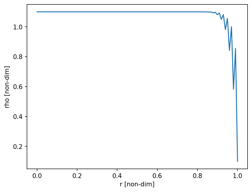
It seems pretty straightforward, yet when it comes to running the code, oscillation rapidly appear, propagating from the outer boundary, where a pressure (i.e. density in the non-dimensional form) gradient builds up, as you can see on the figure below: $rho$ profile at $t=1$ for $\tau=0.1$, $\rho_\infty=0.1$, a time step of 1e-5 and a radial resolution of 100 grid points" /> I had the same issue with an implicit time-stepping, so I thought I'd stick to the simple version. The amplitude of the oscillations is not sensitive to the timestep, and shows little sensitivity to the radial resolution. I am using first order central FD for both equations. I thought it might be an accuracy issue and went for second order central FD for the first equation, which to some extent helped, but not enough. Also, I am not sure about how to go about implementing a second order scheme given my set of boundary conditions; what I did is switch from a central scheme to a forward/backward one when getting to the boundaries, but is doesn't feel very neat.
I can elaborate on the model if needed, I just didn't think it was required, please let me know if I should. What I need is a diagnostic really, because so far I have been trying different ways without much success! The code is provided below.
Thank you for the help!

"""
Non-dimensionalization:
r[non-dim]   = r[m]/R_out
rho[non-dim] = rho[kg/m³]/(deltaP/R/Tref)
p[non-dim]   = p[Pa]/deltaP
v[non-dim]   = v[m/s]
gP[non-dim]  = gP[kg/m³/s]/g0
t[non-dim]   = t[s]/tau_g

Timescales:
tau_g = R/M*T*deltaP/g0
tau_p = viscosity/permeability*R_out^2/deltaP

The physical parameter is tau_g/tau_p,
which quantifies the gas production
time-scale compared to the pressure
gradient-driven outgassing time-scale.

"""

import numpy as np
import matplotlib.pyplot as plt
import time
import copy

# Parameter
tau_g_tau_p = 0.1
P_out       = 0.1 # aka rho_infinite

# All quantities are non-dimensional
N        = 100               # resolution
r        = np.linspace(0,1,N) # radii
dr       = 1/(N-1)            # radius step
rho      = np.ones(N)*P_out   # density
p        = np.ones(N)*P_out   # pressure
gP       = 1.                 # gas production rate
t_max    = 1                  # final time
dt       = 1e-5               # time-step
t        = 0.                 # initial time

while t<t_max:

    rho_prev   = rho
    res = 1
    tol = 1e-5
    while res > tol:

        ##### Picard iteration #####

        ##### Solve Darcy Equation #####

        # calculate p on the staggered grid
        p_stag = (p[:-1]+p[1:])/2 # pressure on the staggered grid

        # compute Darcy flux CFD from staggered p
        v       = np.zeros(N)                  # initialize Darcy flux vector
        v[0]    = 0                            # center BC
        v[1:-1] = -(p_stag[1:]-p_stag[:-1])/dr # central finite-difference
        v[-1]   = -(P_out-p_stag[-1])/(dr/2)       # outer BC

        # CFL check
        if max(v)*dt>dr:
            raise Warning('Courant criterion not respected')

        ##### Solve Mass Conservation Equation ######
        rho_new = rho
        rho_new[1:-1] += gP*dt - tau_g_tau_p*dt/r[1:-1]**2*(r[2:]**2*rho_prev[2:]*v[2:]-r[:-2]**2*rho_prev[:-2]*v[:-2]) # central finite-difference

        # boundary conditions
        rho_new[0]  = rho_new[1] # center BC
        rho_new[-1] = P_out      # outer BC

        ##### Perfect gas law #####
        p = rho_new # non-dimensonal rho and p are the same
    
        # calculate residuals
        res = np.linalg.norm(rho-rho_new)
        rho = rho_new

    t += dt # time increment

# Plot final state
plt.figure()
plt.plot(r,p,label=r'$dt$='+str(dt)+',N='+str(N))
plt.xlabel('r [non-dim]')
plt.ylabel('rho [non-dim]')

Answer 1

Thank you for the tip whpowell96, I did as you suggested and it works fine. I also got inspired by this question. Here is exactly what I've done:

• recast the two equations as one: $$\frac{\partial\rho}{\partial t}-\tau\frac{1}{r^2}\frac{\partial}{\partial r}\left(r^2\rho\frac{\partial\rho}{\partial r} \right)=g_P$$ i.e., making use of $\rho\frac{\partial\rho}{\partial r}=\frac{1}{2}\frac{\partial\rho^2}{\partial r}$: $$\frac{\partial\rho}{\partial t}-\tau\left(\frac{2}{r}\frac{\partial\rho^2}{\partial r}+\frac{\partial^2\rho^2}{\partial r^2} \right)=g_P$$
• then apply central finite difference for the first and second order derivative of $\rho^2$

It is straightforward for an explicit time-stepping, probably more complex for implicit. But explicit is fine for me. Here is the solution code:

"""
Non-dimensionalization:
r[non-dim]   = r[m]/R_out
rho[non-dim] = rho[kg/m³]/(deltaP/R/Tref)
p[non-dim]   = p[Pa]/deltaP
v[non-dim]   = v[m/s]
gP[non-dim]  = gP[kg/m³/s]/g0
t[non-dim]   = t[s]/tau_g
 
Timescales:
tau_g = R/M*T*deltaP/g0
tau_p = viscosity/permeability*R_out^2/deltaP
  
The physical parameter is tau_g/tau_p,
which quantifies the gas production
time-scale compared to the pressure
gradient-driven outgassing time-scale.

"""

import numpy as np
import matplotlib.pyplot as plt

# Parameter
tau_g_tau_p = 0.01
P_out       = 0.1 # aka rho_infinite

# All quantities are non-dimensional
N        = 20               # resolution
r        = np.linspace(0,1,N) # radii
dr       = 1/(N-1)            # radius step
rho      = np.ones(N)*P_out   # density
p        = np.ones(N)*P_out   # pressure
gP       = 1.                 # gas production rate
t_max    = 10                 # final time
dt       = 1e-2               # time-step
t        = 0.                 # initial time

start = time.time()
while t<t_max:

    # outer BC
    rho[-1] = P_out

    # FD for non-linear function rho**2
    rho[1:-1] += tau_g_tau_p*dt*((rho[2:]**2-2*rho[1:-1]**2+rho[:-2]**2)/2/dr \
                                +(rho[2:]**2-rho[:-2]**2)/2/dr/r[1:-1])       \
                                +gP*dt

    # inner BC
    rho[0] = rho[1]

    # CFL check
    v = -np.gradient(rho)
    if max(v)*dt>dr:
       raise Warning('Courant criterion not respected')

    t += dt # time increment

# Plot final state
plt.plot(r,rho,label=r'$dt$='+str(dt)+',N='+str(N))
plt.xlabel('r [non-dim]')
plt.ylabel('rho [non-dim]')