How to solve three coupled differential equations in python using RK-4 and shooting method? or using solve_bvp?

Question

I am trying to solve three coupled differential equations in Python. I am using RK-4 techniques with Shooting method. I am trying to plot the f and N functions.

import numpy as np
import matplotlib.pyplot as plt
from scipy.optimize import fsolve

alpha = 0.1

def F(r, f, v, N, sig):
    g = np.sin(f)
    h = np.cos(f)
    i = np.sin(2 * f)


    dfdr = v
    dNdr = -(alpha*r**2 * N * v**2 *(r**2 + 2 * g**2)+alpha * g**2 * (g**2 +2* r**2) + r**2*(N-1))/r**3
    dsigdr = ( alpha * sig * v**2 * (r**2 + 2 * g**2)) / r
    
    f1= v*((2 * dsigdr * g**2)/(sig * r**2)+(2 * dNdr * g**2)/(N * r**2)+((dsigdr)/sig +dNdr / N + 2 / r))
    dvdr = -(f1 -i/(N * r**2)+(-(2 * g**3 * h)/(N * r**4)+(v**2 * i)/r**2)) / (1 + (2 * g**2) / r**2)
    
    return [dfdr, dNdr, dsigdr, dvdr]

def rk4(F, r_range, f0, v0, N0, s0, h):
    r_values = np.arange(r_range[0], r_range[1], h)
    f_values = np.linspace(f0, 0, len(r_values))
    v_values = np.linspace(v0, 0, len(r_values))
    N_values = np.linspace(N0, 1, len(r_values))
    S_values = np.linspace(s0, 1, len(r_values))

    for i in range(1, len(r_values)):
        r = r_values[i-1]
        f = f_values[i-1]
        v = v_values[i-1]
        N = N_values[i-1]
        sig = S_values[i-1]
    
        k1f, k1v, k1N, k1S = F(r, f, v, N, sig)
        k2f, k2v, k2N, k2S = F(r + 0.5*h, f + 0.5*k1f*h, v + 0.5*k1v*h, N + 0.5*k1N*h, sig +0.5*k1S*h)
        k3f, k3v, k3N, k3S = F(r + 0.5*h, f + 0.5*k2f*h, v + 0.5*k2v*h, N + 0.5*k2N*h, sig +0.5*k2S*h)
        k4f, k4v, k4N, k4S = F(r + h, f + k3f*h, v + k3v*h, N + k3N*h, sig + k3S*h)
    
        f_values[i] = f + ((k1f + 2*k2f + 2*k3f + k4f)*h) / 6
        v_values[i] = v + ((k1v + 2*k2v + 2*k3v + k4v)*h) / 6
        N_values[i] = N + ((k1N + 2*k2N + 2*k3N + k4N)*h) / 6
        S_values[i] = sig + ((k1S + 2*k2S + 2*k3S + k4S)*h)/ 6
    
    return r_values, f_values, v_values, N_values, S_values

rmin = 0.001
rmax = 4
r_range=[rmin, rmax]
h = 0.00001

def objective(u):

    v0, s0 = u
    r_values, f_values, v_values, N_values, S_values = rk4(F, r_range, np.pi, v0, 1, s0, h)
    y1 = f_values[-1]
    y2 = S_values[-1]
    print(f"Objective results: y1={y1}, y2={y2}")

    return [y1 , y2 - 1]

initial_guess=[-0.478, -1.216]
v1 = fsolve(objective, initial_guess, xtol=1e-8)
print("The initial values of v0 and sig0 given by fsolve:", v1[0], " and ", v1[1])

r_values,  f_values, v_values, N_values, S_values = rk4(F, [rmin, rmax], np.pi, v1[0], 1, v1[1], h)
y3 = f_values[-1]
y4 = S_values[-1]
print("The value of f and sig at outer boundary is:", y3, y4)

if np.abs(y3) < 1e-6 and 1<= y4 <1.1:
    print("Boundary condition f(rmax) = 0 is satisfied, and the value of f at outer boundar is:", y3)
    print("Boundary condition sig(rmax) = 0 is satisfied, and the value of sig at outer boundar is:", y4)
else:
    print("The solutions did not converge")

plt.figure(figsize=(14, 10))
plt.plot(r_values, f_values, label='f(r)')
plt.plot(r_values, N_values, label='N(r)')
plt.title(r"$\alpha=0.1$")
plt.xlabel('r')
plt.grid()
plt.legend()
plt.show()

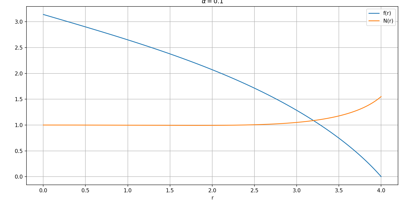
But the nature of the plot is completely different from my expectations. The output is

Objective results: y1=0.000372840219254553, y2=1.0001907509516712
Objective results: y1=0.000372840219254553, y2=1.0001907509516712
Objective results: y1=0.000372840219254553, y2=1.0001907509516712
Objective results: y1=0.00037294172854991653, y2=1.0001906882951273
Objective results: y1=0.000372824083910513, y2=1.0001907727358128
Objective results: y1=1.8398001535383646e-07, y2=0.9999999172810013
Objective results: y1=1.1072732970996606e-11, y2=1.0000000000024691
Objective results: y1=2.1284157569008075e-12, y2=0.9999999999969905
Objective results: y1=1.1784771089214975e-13, y2=0.9999999999997673
The initial values of v0 and sig0 given by fsolve: -0.4780664768861783  and  -1.2166450055671914
The value of f and sig at the outer boundary is: 1.1784771089214975e-13 0.9999999999997673
The solutions did not converge

As you see the value of sig at the outer boundary is almost one (0.9999999999997673).

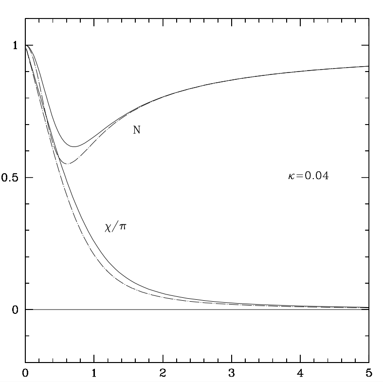
1. [This is the nature of the plot as expected]

2. [This is the plot I am getting]

3. [These are the three coupled differential equations with boundary conditions]

I also tried the above code with a smaller value of h (=0.000001) and different values of rmin, rmax, alpha and initial_guess but the result was the same.

I also tried to solve the problem using solve_bvp. Here is the code using solve_bvp

import numpy as np
from scipy.integrate import solve_bvp
import matplotlib.pyplot as plt


alpha = 0.1


def F(r, f):
    #f, v, N, sig = S
    g = np.sin(f[0])
    h = np.cos(f[0])
    i = np.sin(2 * f[0])
    
    #dfdr = v
    dNdr = -( alpha * r**2 * f[2] * f[1]**2 * (r**2 + 2* g**2) +  alpha * g**2 * (g**2 +2* r**2) + r**2 * (f[2] - 1)) / r**3
    dsigdr = ( alpha * f[3] * f[1]**2 * (r**2 + 2 * g**2)) / r
    ter1=((dsigdr) / f[3] + dNdr / f[2] + 2 / r  +(2 * dsigdr * g**2) / (f[3] * r**2) + (2 * dNdr* g**2) / (f[2] * r**2))
    dvdr = -((f[1] * ter1 - i / (f[2] * r**2)) + (-(2 * g**3 * h) / (f[2] * r**4) + (f[1]**2 * i) / r**2)) / (1 + (2 * g**2) / r**2)
    
    return np.vstack((f[1], dvdr, dNdr, dsigdr))


def bc(fa, fb):
    return np.array([fa[0]-np.pi, fb[0]-0, fa[2]-1, fb[3]-1])

rmin = 0.001
rmax = 5
x = np.linspace(rmin, rmax, 100000)


y=np.ones([4, x.size])
y[0, :] = np.linspace(np.pi, 0, x.size)
y[1, :] = np.linspace(-0.2, 0, x.size)

y[2, :] = np.linspace(1, 1, x.size)
y[3] = np.ones(x.size)  


sol = solve_bvp(F, bc, x, y, tol=1e-8, max_nodes=100000, verbose=2)

if sol.success:
    print("Solution converged")
else:
    print("Solution did not converge")
    print("Residuals:", sol.message)
    print("Residuals max:", np.max(sol.rms_residuals))


print(sol)
#Plot the solutions
plt.figure(figsize=(14, 10))
plt.plot(sol.x, sol.y[0], label='f(r)')
#plt.plot(sol.x, sol.y[1], label='V(r)')
plt.plot(sol.x, sol.y[2], label='N(r)')
plt.xlabel('r')
plt.grid()
plt.legend()
plt.show()

When I am using solve_bvp, I am getting the following error

Iteration    Max residual  Max BC residual  Total nodes    Nodes added  
       1          1.06e+00       3.41e-21        100000        (199998)    
Number of nodes is exceeded after iteration 1. 
Maximum relative residual: 1.06e+00 
Maximum boundary residual: 3.41e-21
Solution did not converge
Residuals: The maximum number of mesh nodes is exceeded.
Residuals max: 1.0570652692628755
       message: 'The maximum number of mesh nodes is exceeded.'
         niter: 1
             p: None
 rms_residuals: array([4.25858920e-01, 2.54417888e-01, 1.98041640e-01, ...,
       6.12622641e-05, 6.11022248e-05, 6.09430998e-05])
           sol: <scipy.interpolate._interpolate.PPoly object at 0x000001B21E651DF0>
        status: 1
       success: False

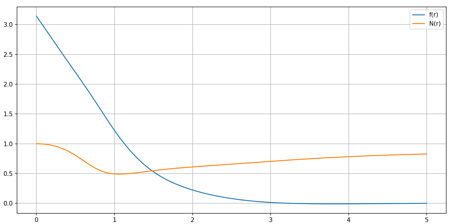
The plot using solve_bvp is better but the success status is false.

[This plot is done using solve_bvp]

Answer 1

I don’t think anyone can answer this question intelligently without debugging your code. That being said, it is unsurprising that scipy’s method performs better. If you want your implementation to work correctly consider isolating and testing individual components on simple problems with answers that are easy to verify. If everything tests well and it still isn’t working, I would consider using a time integration scheme from script as well. There is really no reason to ever write your own RK method in Python except for a homework assignment. If all you want is a solution, solve_bvp with fewer nodes/higher maximum nodes seems like a safe bet.